Moment tensor analysis is a topic that carries a decent level of uncertainty and confusion for many people. So I’m going to lay it out as simply as I can. For this post, I’m not going to go into too many details on how moment tensors are actually calculated. But, I’m going to summarise the things I think are most important for geotechnical engineers to know for interpreting moment tensor results.
OK, so, what is a moment tensor?
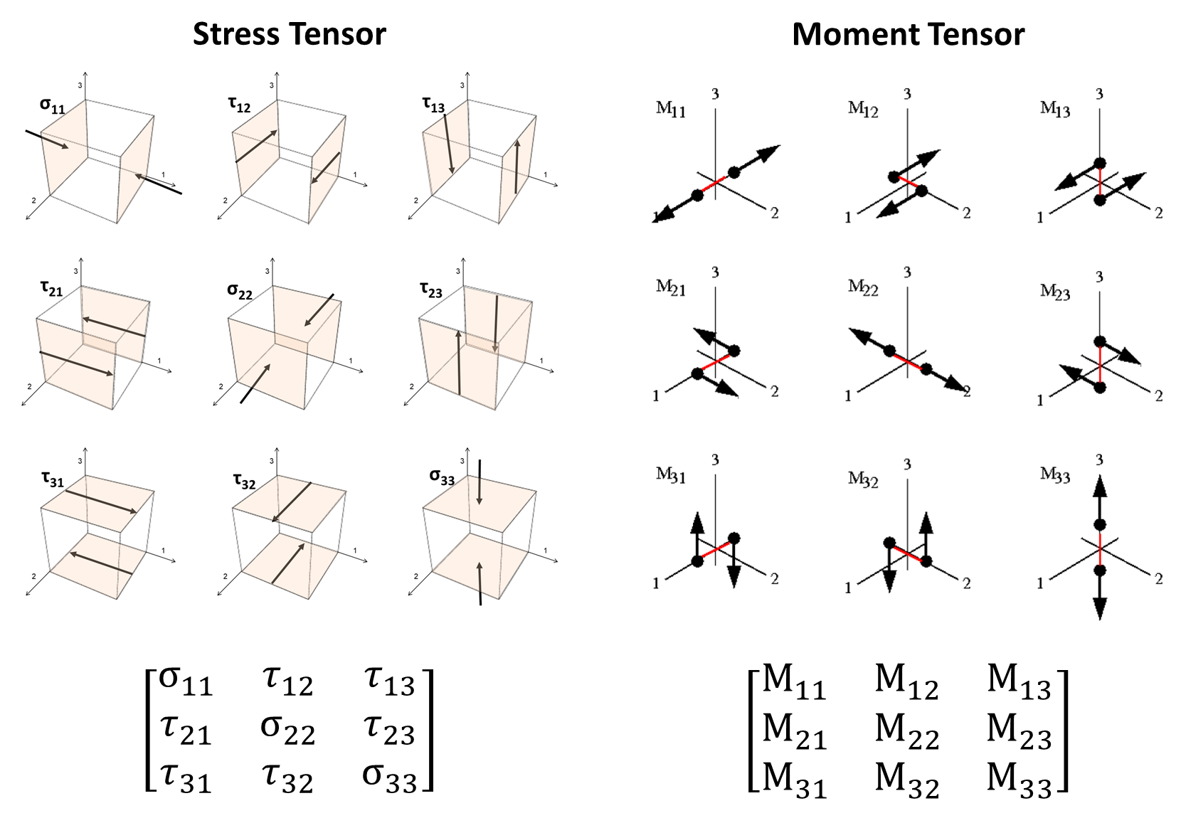
A moment tensor is a representation of the source of a seismic event. The stress tensor and the moment tensor are very similar ideas. Much as a stress tensor describes the state of stress at a particular point, a moment tensor describes the deformation at the source location that generates seismic waves.
You can see the similarity between the stress and moment tensors in the figure below. The moment tensor describes the deformation at the source based on generalised force couples, arranged in a 3 x 3 matrix. Although, the matrix is symmetric so there are only six independent elements (i.e. M12 = M21). The diagonal elements (e.g. M11) are called linear vector dipoles. These are equivalent to the normal stresses in a stress tensor. The off-diagonal elements, are moments defined by force couples (moments and force couples discussed in previous blog post).
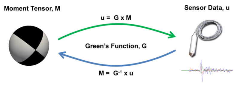
Producing a moment tensor of a seismic event requires the Green’s function. This function computes the ground displacement recorded by the seismic sensor based on a known moment tensor (the forwards problem). A moment tensor inversion is when the inverse Green’s function is used to find the source moment tensor based on sensor data.
Sure… but what’s with the beach balls?
It’s pretty hard to interpret a 3 x 3 matrix of numbers, so moment tensors are usually displayed as beach balls, either 2D or 3D. I will mostly discuss the 3D case; the 2D diagram is just a stereonet projection of the 3D beach ball.
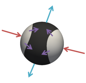
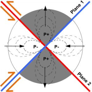
The construction of a beach ball diagram is very simple. For each point on the surface of a sphere, the moment tensor describes the magnitude and direction of the first motion. If the direction of motion is inwards, towards the source, the surface is coloured white (red arrows). If the direction of motion is outwards, away from the source, the surface is coloured black (blue arrows). Where there is a border between black and white on the beach ball surface, the direction of motion is tangential (purple arrows). The direction of motion across the border is white-to-black.
The figure below shows the first ground motion on the beach ball surface, split into radial and tangential components. The lengths of the radial and tangential arrows are proportional to the strength of the P and S waves respectively. P-waves generally emanate strongest from the middle of the white and black regions. S-waves emanate strongest from the black-white borders.

The location of the pressure and tension axes can be confusing. If you look at the S-waves diagram, the tension axis is in the compressional quadrant. However, it does make more sense from the P-waves diagram. The black/white convention can also be counter-intuitive for some. ‘Black’ holes pull things inwards, the sun radiates ‘white’ light outwards, but the beach ball diagram is the opposite of that. I’m sorry I don’t know why this is the convention. Perhaps seismologists are Star Wars fans… Vader wants Luke to come to the dark side, and so this is the movement direction that he is tempted towards… that’s all I got ?.
Right, but what can I learn about the event mechanism?
Even with the beach ball diagram, it can still be hard to interpret the geological or physical mechanism of the event. This is why the moment tensor is often decomposed into its constituent elementary source mechanisms. To decompose the moment tensor, the matrix is rotated to zero the off-diagonal elements. This is just like finding the principal axes of a stress tensor, by zeroing the shear elements and leaving the normal stresses. So, every moment tensor can be expressed as three linear vector dipoles (orthogonal), rotated to a particular orientation. These three dipoles are referred to as the P (pressure), B (or N, neutral or null) and T (tension) principal axes.
Isotropic source
In combination, the three dipoles either result in an overall expansion or a contraction of the source volume. If the source is explosive, the largest dipole direction is the T axis and the smallest dipole is the P axis. These are reversed for an implosive source. Although, for a pure isotropic source the axis orientations have no meaning.
The isotropic component is the portion of the tensor that represents a uniform volume change. Only P-waves radiate from a purely isotropic source. A positive isotropic component is an expansion/explosion. This can be a confined blast or possibly rock bulking. A negative isotropic component is a contraction/implosion. Any pillar burst, buckling or rock ejecting into a void will likely appear as an implosion, given the path of the recorded waves around the void, all first motions will be towards the source.
Deviatoric source
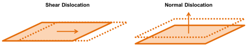
When the isotropic component is removed from the moment tensor, the remainder is the deviatoric component. The deviatoric tensor results in displacement that has zero net volume change, i.e. equal movement in, equal movement out. The underlying geological process to the deviatoric component is a general dislocation of a fault. The general dislocation can be a mix of shear and normal dislocation (although still with no net volume change). To better interpret the relative proportions of shear and normal displacement, the deviatoric component can be decomposed into the DC and CLVD elemental sources.
Double Couple (DC) source
The DC source is a pure shear dislocation. It is referred to as a double couple because there are two force couples and two (alternate) fault plane orientations that equally model the expected displacement. This notion was discussed in a previous post. The shear direction on the fault is from white-to-black. You can review the orientation of the two planes in relation to your site geology. It may be the case that one of the planes makes more sense than the other or you can find the specific structure.
A pure DC source has two equal and opposite linear vector dipoles. The third dipole is zero (B or null axis). The embedded video shows the direction of first motions from a pure DC source. As mentioned already, motion is inwards for the white regions, outwards for the black regions and tangential across black-white borders. Radial movement radiates P-waves, tangential movement radiates S-waves.
Compensated Linear Vector Dipole (CLVD) source
The CLVD source is a normal dislocation on a plane. The normal displacement from one linear vector dipole is ‘compensated’ (hence the name) by opposing displacement from the other two linear vector dipoles so that there is no net volume change.
For a positive CLVD source, a single tensile dipole is compensated by two compressive dipoles.
Vice-versa for a negative CLVD source.
A pure CLVD source would imply a Poisson’s ratio of 0.5, which is more like chewing gum or toothpaste than rock. So there is no geological example of a pure CLVD source. Although, it can make sense as a mixed source event; i.e. part isotropic, part CLVD. This event mechanism may be dominant for confined pillar crushing events. The Hudson chart indicates two key points that are a combination of isotropic and CLVD sources. A single linear vector dipole (other two dipoles are zero) decomposes to a one-third isotropic source, two-thirds CLVD. A pure tensile crack mechanism decomposes to a source 55% explosive, 45% positive CLVD.
The Hudson chart is a useful tool to visualise the moment tensor decomposition, seeing the relative proportions of the isotropic, DC and CLVD elemental sources. The vertical axis is the isotropic component, from -100% (implosion) to 100% (explosion). The horizontal axis is the deviatoric decomposition, from +100% to -100% CLVD, with 100% DC in the centre (0% isotropic, 0% CLVD). The outer border is the 0% DC line.

Final comments
There are many factors that can lead to uncertainty in determining the first motions of waves recorded at sensors and the final moment tensor solution. Seismic waves travelling through the rock mass divert around mining voids and go through numerous refractions, reflections and superimpositions. Noise at the sensor site can also influence the first motion analysis and the solution can also be very sensitive to poor P and S picks. Good moment tensor solutions require a sensor array that is well dispersed, covering the focal sphere in all three dimensions.
Be aware that each moment tensor solution is not going to be of equal quality, particularly small events with few sensors used. Your seismic service provider should provide you with some measure of solution accuracy to help assess this. This might be based on an assessment of the sensor configuration or a misfit analysis between the observed waveforms and the theoretical waveforms generated synthetically from the moment tensor. In general, it is better to look at trends and a convergence of evidence across multiple events rather than a single moment tensor solution. Even if you are investigating a single large event, it is probably worth reviewing the mechanisms of aftershocks and previous events in the area.
It is important not to jump blindly to the nodal plane solutions and to consider the decomposition of the moment tensor in your analysis. If the source is only 5-10% DC, the nodal planes are not very significant. The P, B, T axis are also less important for strongly isotropic sources so keep that in mind for stereonet analysis.
And one last warning about CLVD components. In tests where random noise is added to an initial noise-free, moment tensor inversion of a pure DC source, the noise serves to increase the CLVD component. So it is hard to be sure when CLVD shows up in a solution that it isn’t just noise related. In fact, seismologists often evaluate the accuracy of a moment tensor solution by how large the CLVD component is. A good solution would have a low CLVD component. This is earthquake seismology though so the range of rock mass mechanisms is less diverse than the mining environment, DC is often an assumption for earthquakes.
Anyway, hopefully that clears up at least some of the mystery around moment tensors. Feel free to contact support with any questions. For those looking to read up further I recommend this manual by Dahm & Krüger (2014) and the references therein. They go into much more detail on alternate decompositions and the moment tensor inversion process.